Use of censored bivariate normal model function for yield gap analysis • BLA

Introduction

The censored bivariate normal model (Lark and Milne, 2016) is a statistical method to fit the boundary line to data. It fits the boundary line using the maximum likelihood approach on a censored bivariate distribution. This removes the subjectivity associated with the other boundary line fitting methods ( bolides, Binning and quantile regression) of selecting boundary points to which the boundary line is fitted or specifying an arbitrary quantile to model. It also gives evidence for the presence of boundary in a data set against a bivariate normal null distribution. This method has been previously used to fit boundary lines to data on nitrous oxide emission as a function of soil moisture (Lark and Milne, 2016) and, wheat yield as a function of nutrient concentration (Lark et al. 2020). An R package, BLA, contains exploratory and boundary fitting functions that can be used in the process of fitting a boundary line to data using the censored bivariate normal model. This vignette gives a step by step process for fitting the boundary line and subsequent post-hoc analysis. In this demonstration, the data set soil will be used and boundary line analysis will be carried out on soil P and pH.

Load the BLA package

Load the BLA package using the library() function. In addition, the aplpack package is also loaded. The aplpack package contains the bagplot() function which is used to identify outliers in a data set.

library(BLA)

library(aplpack)

Yield gap analysis using boundary lines

The data that is going to be used for this is called the soilwhich is part of the BLA package. It contains measures of wheat yield on farms from different parts of the UK and its associated soil properties pH and phosphorus. The process of yield gap analysis involves two step that include (1) fitting the boundary line and (2) determining the most limiting factor. We will first fit the boundary line to soil P and then to pH after which the most limiting factor will be determined.

data("soil")

Soil P boundary line fitting

Data exploration

Exploratory analysis is an essential initial step in fitting a boundary line to data. This step ensures that the assumptions for the censored bivariate normal model are met. Three exploratory procedures are performed on the data which include (1) Assessing the plausibility of normality of variables, (2) Removal of outliers, and (3) Testing for evidence of boundary in the data.

1. Assessing normality of independent and dependent variable

Boundary line model fitting using cbvn() requires that the independent (x) and dependent (y) variables are normally distributed albeit with censoring of the variable y. The summastat() function gives summary statistics of the distribution of a variable. The octile skewness is a robust measure of skew, and we expect its absolute value to be less than 0.2 for a normally distributed variable. We also assess plots of the data, bearing in mind that the dependent variable may be subject to censoring of large values under our target model.

x<-soil$P
y<-soil$yield

#Distribution of the x variable

summastat(x)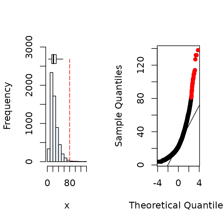

#>         Mean Median Quartile.1 Quartile.3 Variance       SD Skewness
#> [1,] 25.9647     22         16         32 207.0066 14.38772 1.840844
#>      Octile skewness Kurtosis No. outliers
#> [1,]       0.3571429 5.765138           43

summastat(log(x))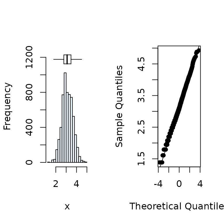

#>          Mean   Median Quartile.1 Quartile.3  Variance        SD  Skewness
#> [1,] 3.126361 3.091042   2.772589   3.465736 0.2556936 0.5056615 0.1297406
#>      Octile skewness    Kurtosis No. outliers
#> [1,]      0.08395839 -0.05372586            0

x<-log(x) # since x required a transformation to assume it is from a normal distribution.

#Distribution of the y variable

summastat(y)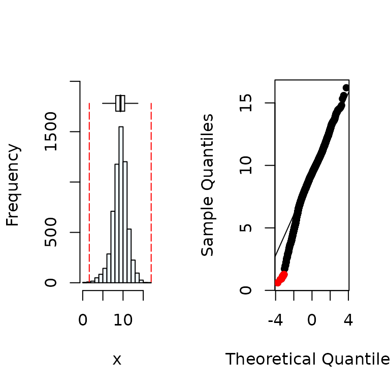

#>          Mean  Median Quartile.1 Quartile.3 Variance       SD   Skewness
#> [1,] 9.254813 9.36468   8.203703   10.39477 3.456026 1.859039 -0.4819805
#>      Octile skewness Kurtosis No. outliers
#> [1,]     -0.05793291 1.292635            7

2. Removal of outliers

Boundary line analysis is sensitive to outlying values and hence it is required that they are identified and removed. This can be done using the bagplot() function of the aplpack package. The bag plot, a bivariate box plot, has four main components, (1) a depth median (equivalent to the median in a box plot) which is represents the centre of the data set, (2) The bag which contains 50% of the data points (eqiuavalent to the interquartile range), (3) a ‘fence’ that separates probable outliers, (4) a loop which contains points outside the bag but are not outliers.


# Create a dataframe containing x and y

df<-data.frame(x,y)

# Input the dataframe into the bagplot() function

bag<-bagplot(df,show.whiskers = FALSE, ylim=c(0,20),create.plot = FALSE)

# Combine data points from "bag" and within the loop i.e. exclude the outliers

dat<-rbind(bag$pxy.bag,bag$pxy.outer)

# Output is a matrix, we can pull out x and y variables for next stage 

x<-dat[,1] 
y<-dat[,2]

3. Testing data for presence of boundary

If a boundary exists in a data set, it is expected that there will be some clustering of observations at the upper edges of the data cloud compared to a bivariate normally distributed data for which data points at the upper edges are sparse because of the small probability density . A boundary can be assumed in a data set if there is evidence of clustering at the upper edges. The expl_boundary() function, which is based on the convex hull, can be used to access presence of boundary (Miti et al, 2024). This function checks probability of the observed clustering if it came from a bivariate normal distribution (p-value).


expl_boundary(x,y) # may take a few minutes to complete

From the results, the probability (p-value) of the having points close to each other as in our data if it came from a bivariate normally distributed data is less than 5%. Therefore, there is evidence of bounding effects in the data in the right and left sections of the data. Note that, in the plot, the data is split into right and left sections to get more information on the clustering nature of points.

Fitting the boundary line to data

The exploratory tests indicated that the data provide evidence of a boundary, outliers have been identified and removed, and the variables x and y are normally distributed. We therefore proceed to fit a boundary line model to the data set using the censored bivariate normal model. The function cbvn() fits the boundary line to the data. For more information about the arguments of this function, check

?cbvn

Argument values for the function cbvn() need to be set . Firstly, create a data-frame containing x and y, called data.

data<-data.frame(x,y) #This is an input dataframe containing the variables

Secondly, the cbvn() requires initial starting values, start, which are parameters of the boundary line (the censor) and the bivariate normal distribution. Starting values of the boundary line depend on the model that one wishes to fit to the data (see options in ?cbvn) . In this case, we shall fit a linear+plateau model (lp) and hence the parameters are the plateau value and the intercept and slope of the linear component. The boundary line start values can be obtained using the function startValues(). For more information on the startValues() function run the code ?startValues. With a scatter plot of y against x active in the plot window in R, run the function start.values("lp"), then click on the plot, the point you expect to be the lowest and the largest response of a linear model at the boundary. Note that starting values for other models can be determined by changing the model name from “lp” to the desired models (see ?startValues help file).

plot(x,y)

startValues("lp")

Next, determine the parameters of the bivariate normal distribution which include the means of the x and y variables, standard deviation of the x and y variables, and the correlation of x and y.

mean(x) 
#> [1] 3.125969
mean(y) 
#> [1] 9.28862
sd(x) 
#> [1] 0.5005755
sd(y) 
#> [1] 1.728996
cor(x,y)
#> [1] 0.0346758

#The parameters of the boundary line and the data can be combined in a #vector start in the order 
#start<-c(intercept, slope, max response, mean(x), mean(y), sd(x), sd(y), cor(x,y))

Another important argument is the standard deviation of the measurement error, sigh, of the response variable y. In some cases this might be estimated from observations of analytical duplicates, or experiments to determine measurement error for variables such as crop yield (e.g. Kosmowski et al. 2021). However, in cases when this is not available, it can be estimated using different options. One option of estimation is to use a variogram if the location data for samples is available. In that case, nugget variance which is the unexplained short distance variations can be taken as an estimate of the measurement error. If this is not possible, a profiling procedure can be done. This is done by fitting a proposed model using a varied number of sigh values while keeping the rest of the model parameters constant. The log-likelihood values of the model for each sigh are determined and the value that maximizes the likelihood can be selected from the log-likelihood profile. This can be implemented using the ble_profile() function. For more information on this function run

?ble_profile

The possible sigh values can be set to 0.5, 0.7 and 0.8 and we can check the likelihood profile.


sigh=c(0.5,0.7,0.8)
ble_profile(data,start,sigh,model = "lp") # may take a few minutes to run for large datasets

From the likelihood profile, the sigh that maximizes the likelihood is around 0.65. We can use this for the value of sigh. Now that all the arguments required for cbvn() function are set, the boundary line can be fitted

start<-c(4,3,13.6,3,9,0.50,1.9,0.05)

model1<-cbvn(data,start=start,sigh=0.7,model = "lp", xlab=expression("P /log ppm"), ylab=expression("Yield /t ha"^{-1}), pch=16, col="grey")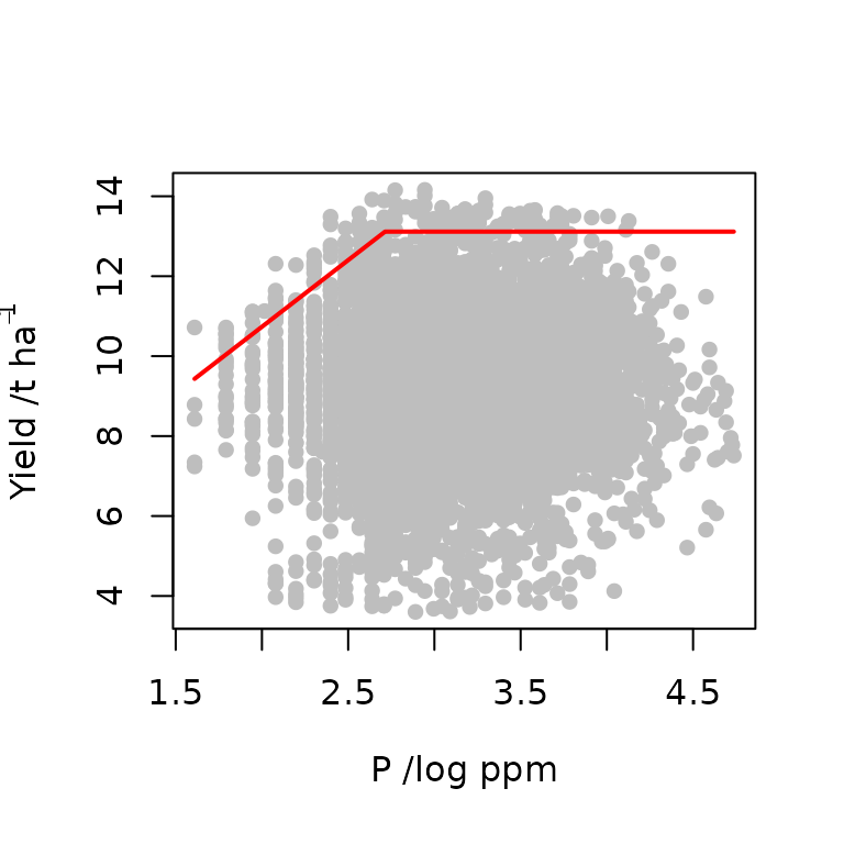


model1
#> $Model
#> [1] "lp"
#> 
#> $Equation
#> [1] y = min (β₁ + β₂x, β₀)
#> 
#> $Parameters
#>          Estimate Standard error
#> β₁     4.06696830    1.062543187
#> β₂     3.33394003    0.483101081
#> β₀    13.11509466    0.162435745
#> mux    3.12596804    0.006451141
#> muy    9.29877801    0.022677786
#> sdx    0.50053541    0.004550540
#> sdy    1.60137534    0.018125877
#> rcorr  0.03013859    0.014294338
#> 
#> $AIC
#>             
#> mvn 32429.55
#> BL  32399.25

The boundary line is fitted and the parameters together with their corresponding standard error values are obtained. However, there is one question that needs to be addressed before we proceed,

Is the boundary line ideal for this data?

While fitting the BL model to the data, the cbvn() also fits a bivariate normal model with no boundary and calculates it AIC value. From our output, the AIC value of the BL model is lower than that of the bivariate normal model. Therefore, the BL model is appropriate. The parameters of the boundary line can now be used to predict the boundary yield given the value of P.

The function predictBL() in the BLA package can be used for this. For more information about the function, see

?predictBL

We need to predict the largest expected yield for each point given the soil P. We will replace any missing values with the mean value of P.


xp<-log(soil$P) # let xp be the P content in our dataset
xp[which(is.na(xp)==T)]<-mean(xp,na.rm=T)
P<-predictBL(model1,xp)

We can proceed to the next variable pH using the same procedure.

Soil pH boundary line fitting

Data exploration

1. Testing for normality of independent and dependent variable

x<-soil$pH
y<-soil$yield

# Distribution of the x variable

summastat(x)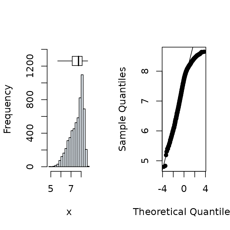

#>          Mean Median Quartile.1 Quartile.3  Variance        SD   Skewness
#> [1,] 7.566206   7.74       7.12        8.1 0.4344038 0.6590931 -0.7968046
#>      Octile skewness    Kurtosis No. outliers
#> [1,]      -0.3594771 -0.07912815            0

2. Removal of outliers

 
# Create a dataframe of x and y which is an input into the bagplot() function

df<-data.frame(x,y) 

# Input the dataframe into the bagplot() function.

bag<-bagplot(df,show.whiskers = FALSE, ylim=c(0,20),create.plot = FALSE)

# Combine data points from "bag" and within the loop

dat<-rbind(bag$pxy.bag,bag$pxy.outer)

# Output is a matrix, we can pull out x and y variables for next stage 

x<-dat[,1] 
y<-dat[,2]

3. Testing data for presence of boundary

This was already done using P and boundary existence was confirmed

Fitting the boundary line to data

From the exploratory tests, they indicated that the data provides evidence of boundary existence, outliers have been identified and removed, and the variables x and y are normally distributed. We therefore, proceed to fit a boundary line model to the data set using the censored bivariate normal model. The function cbvn() fits the boundary line to the data.

We determine the argument values for the function cbvn() as before . Firstly, create a data-frame containing x and y, called data.

data<-data.frame(x,y) #This is an input dataframe containing the variables

Secondly, the cbvn() requires initial starting values, start, which are parameters of the boundary line (the censor) and the bivariate normal distribution. In this case, we shall fit a linear+Plateau model (lp) and hence the parameters are the plateau value and the intercept and slope of the linear component. With a scatter plot of y against x active in the plot window in R, run the function start.values("lp"), then click on the plot, the point you expect to be the lowest and the largest response of a linear model at the boundary. Note that starting values for other models can be determined by changing the model name from “lp” to the desired models (see ?startValues help file)

plot(x,y)

startValues("lp")

mean(x) 
#> [1] 7.569203
mean(y) 
#> [1] 9.277917
sd(x) 
#> [1] 0.656315
sd(y) 
#> [1] 1.755941
cor(x,y)
#> [1] 0.1169399

#The parameters of the boundary line and the data can be combined in a #vector start in the order 
#start<-c(intercept, slope, max response, mean(x), mean(y), sd(x), sd(y), cor(x,y))

start<-c(-9,3, 13.5,7.5,9,0.68,2.3,0.12)

The standard deviation of the measurement error, sigh was already determine as 0.7. Now that all the arguments required for cbvn() function are set, the boundary line can be fitted


model2<-cbvn(data,start=start,sigh=0.7,model = "lp", xlab=expression("pH"), ylab=expression("Yield /t ha"^{-1}), pch=16, col="grey")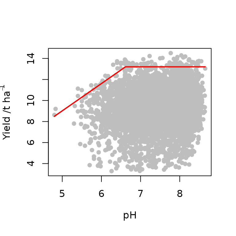


model2
#> $Model
#> [1] "lp"
#> 
#> $Equation
#> [1] y = min (β₁ + β₂x, β₀)
#> 
#> $Parameters
#>         Estimate Standard error
#> β₁    -3.9496784    0.625843951
#> β₂     2.5933540    0.107681571
#> β₀    13.2048773    0.173877733
#> mux    7.5692058    0.008439500
#> muy    9.2839579    0.022826649
#> sdx    0.6562763    0.005967654
#> sdy    1.6239692    0.018077098
#> rcorr  0.1233113    0.014184125
#> 
#> $AIC
#>             
#> mvn 35962.04
#> BL  35946.16

The boundary line is fitted and the parameters together with their corresponding standard error values are obtained. From our output, the AIC value of the BL model is lower than that of the bivariate normal model. Therefore, the BL model is appropriate. The parameters of the boundary line can now be used to predict the boundary yield given the value of pH using the function predictBL(). We need to predict the largest expected yield for each farm given the soil pH. We will replace any missing values with the mean value of pH.


xpH<-soil$pH # let xpH be the P content in our dataset
xpH[which(is.na(xpH)==T)]<-mean(xpH,na.rm=T)
pH<-predictBL(model2,xpH)

Determination of most limiting factor

The boundary line analysis has been used to determine the most limiting factor in many yield gap analysis studies. This is according to the von Liebig (1840) law of the minimum

$$ y={\rm min}(f_1(x_1),f_2(x_2),...,f_n(x_n)) $$

In the BLA package, the function limfactor() can be used to determine the most limiting factor at each point. For more information on the function, see

?limfactor

For the two soil properties in our dataset, the most limiting factor for each data point is determined as


Limiting_factor<-limfactor(P,pH) # This produces a list of length 2 containg a vector limiting factors at each pont and the maximum predicted response in the dataset.

Limiting_factors<-Limiting_factor[[1]]

We can check the proportion of cases in which each of the soil properties was limiting

Lim_factors<-Limiting_factors$Lim_factor

barplot(prop.table(table(Lim_factors))*100,
        ylab = "Percentage (%)",
        xlab = "Soil property",
        col = "grey",
        ylim=c(0,90))

axis(side = 1, at = seq(0, 4, by = 1), labels = FALSE, lwd = 1, col.ticks = "white")  
axis(side = 2, lwd = 1)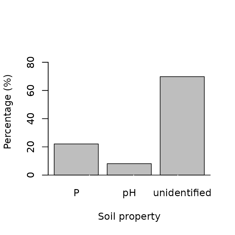

As only two factors were evaluated, most of the yield gap cause was unidentified. This is because there many other factors affecting yield which we did not consider in this case. You can also plot the predicted yield by the most limiting factor against the actual yield.


plot(Limiting_factors$Rs, soil$yield,
     xlab="Predicted yield (ton/ha)",
     ylab="Actual yield (ton/ha)", pch=16, col="grey")

abline(h=Limiting_factor[[2]], col="blue", lty=5, lwd=1)
lines(c(min(Limiting_factors$Rs),max(Limiting_factors$Rs)), 
c(min(Limiting_factors$Rs),max(Limiting_factors$Rs)), 
col="red", lwd=2)

legend("bottomleft",legend = c("Att yield", "1:1 line"),
       lty=c(5,1), col=c("blue", "red"), lwd=c(1, 2), cex = 0.8)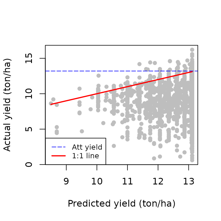

The dashed blue line represents the attainable yield for this particular setting. The 1:1 describes the situations in which the actual yield is equal to the predicted yield by the most limiting factor. The yield gap for each point is equivalent to the vertical distance between the point and the 1:1 line. The points above the 1:1 line are considered to have zero yield gap and their position above the line is only due to measurement error.

Concluding remarks

The censored bivariate normal model has been used to carry out a yield gap analysis. The advantage of using this method over the other boundary line fitting methods is that it is based on statistical principles and it removes the subjectivity associated with selection of bin sizes and the quantile to consider as boundary as it is done in the binning methodology and quantile regression. Furthermore, the uncertainty around the boundary line can also be determined.

References

Kosmowski, F., Chamberlin, J., Ayalew, H., Sida, T., Abay, K., & Craufurd, P. (2021). How accurate are yield estimates from crop cuts? evidence from small-holder maize farms in ethiopia. Food Policy, 102 , 102122. https://doi.org/10.1016/j.foodpol.2021.102122
Lark, R. M., Gillingham, V., Langton, D., & Marchant, B. P. (2020). Boundary line models for soil nutrient concentrations and wheat yield in national-scale datasets.European Journal of Soil Science, 71 , 334-351. https://doi.org/10.1111/ejss.12891
Lark, R. M., & Milne, A. E. (2016). Boundary line analysis of the effect of water filled pore space on nitrous oxide emission from cores of arable soil. European Journal of Soil Science, 67 , 148-159. https://doi.org/10.1111/ejss.12318
Milne, A. E., Wheeler, H. C., & Lark, R. M. (2006). On testing biological data for the presence of a boundary. Annals of Applied Biology, 149 , 213-222. https://doi.org/10.1111/j.1744-7348.2006.00085.x
Miti, C., Milne, A., Giller, K., Sadras, V., & Lark, R. (2024). Exploration of data for analysis using boundary line methodology. Computers and Electronics in Agriculture, 219. https://doi.org/10.1016/j.compag.2024.108794