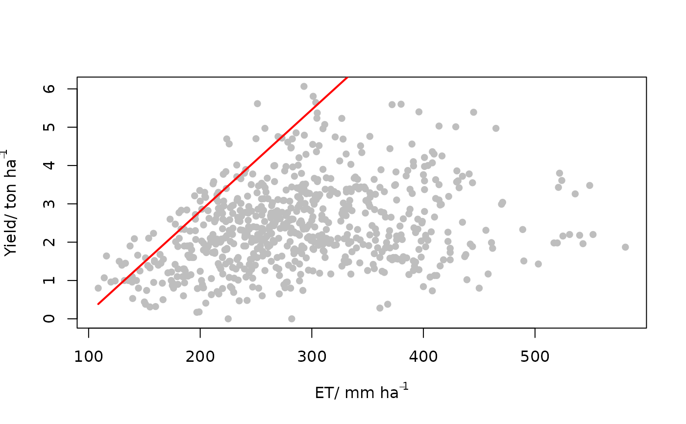
Fitting boundary line using censored bivariate normal model

This function fits a response model to the upper limits of a scatter plot of of x and y to determine the most efficient response of y as a function of x (given a measurement error of y) based on a censored distribution (Milne et al., 2016). The location of censor in the data cloud is determined based on the maximum likelihood approach. This is done using optimization procedure and hence requires some starting guess parameters for the proposed model. It then compares the results with an uncensored normal bivariate distribution to access the appropriateness of the censored model.

Usage

cbvn(data,model="lp", equation=NULL, start, sigh, UpLo="U", optim.method="BFGS",
      Hessian=FALSE, plot=TRUE, line_smooth=1000, lwd=2, l_col="red",...)

Arguments

data

A dataframe with two numeric columns, independent (x) and dependent (y) variables respectively.

model

Selects the functional form of the boundary line. It includes "blm" for linear model, "lp" for linear plateau model, "mit" for the Mitscherlich model, "schmidt" for the Schmidt model, "logistic" for logistic model, "logisticND" for logistic model proposed by Nelder (1961), "inv-logistic" for the inverse logistic model, "double-logistic" for the double logistic model, "qd" for quadratic model and the "trapezium" for the trapezium model. For custom models, set model = "other".

equation

A custom model function writen in the form of an R function. Applies only when argument model="other", else it is NULL.

start

A numeric vector of initial starting values for optimization in fitting the boundary model. Its length and arrangement depend on the suggested model:

For the "blm" model, it is a vector of length 7 arranged as the intercept, the slope, mean of x, mean of y, standard deviation of x, standard deviation of y and the correlation of x and y.
For the "lp" model, it is a vector of length 8 arranged as the intercept, the slope, the maximum or plateau response, mean of x, mean of y, standard deviation of x, standard deviation of y and the correlation of x and y.
For the "mit" model, it is a vector of length 8 arranged as the intercept, shape parameter, the maximum or plateau response, mean of x, mean of y, standard deviation of x, standard deviation of y and the correlation of x and y.
For the "logistic", "inv-logistic" and "logisticND" models, it is a vector of length 8 arranged as scaling parameter, shape parameter, the maximum or plateau value, mean of x, mean of y, standard deviation of x, standard deviation of y and the correlation of x and y.
For the "double-logistic" model, it is a vector of length 11 arranged as scaling parameter, shape parameter, maximum response, maximum response, scaling parameter two, shape parameter two, mean of x, mean of y, standard deviation of x, standard deviation of y and the correlation of x and y.
For the "trapezium" model, it is a vector of length 10 arranged as intercept one, slope one, maximum response, intercept two, slope two, mean of x, mean of y, standard deviation of x, standard deviation of y and the correlation of x and y.
For the "qd" model, it is a vector of length 8 arranged as a constant, linear coefficient, quadratic coefficient,mean of x, mean of y, standard deviation of x, standard deviation of y and the correlation of x and y.
For the "schmidt" model, it is a vector of length 8 arranged the scaling parameter, shape parameter (x-value at maximum response ), maximum response, mean of x, mean of y, standard deviation of x, standard deviation of y and the correlation of x and y.

sigh

Standard deviation of the measurement error.

UpLo

Selects the type of boundary. "U" fits the upper boundary and "L" fits the lower boundary.

optim.method

Describes the method used to optimize the model as in the optim() function. The methods include "Nelder-Mead", "BFGS", "CG", "L-BFGS-B", "SANN" and "Brent".

Hessian

If True, the hessian matrix is part of the output (default is FALSE`).

plot

If TRUE, a plot is part of the output. If FALSE, plot is not part of output (default is TRUE).

line_smooth

Parameter that describes the smoothness of the boundary line. (default is 1000). The higher the value, the smoother the line.

lwd

Determines the thickness of the boundary line on the plot (default is 1).

l_col

Selects the color of the boundary line.

...

Additional graphical parameters as in the par() function.

Value

A list of length 5 consisting of the fitted model, equation form, parameters of the boundary line, AIC (for boundary line model and a null model) and a hessian matrix. Additionally, a graphical representation of the boundary line on the scatter plot is produced.

Details

Some inbuilt models are available for the cbvn() function. The suggest model forms are as follows:

Linear model ("blm") $$y=\beta_1 + \beta_2x$$ where $\beta_1$ is the intercept and $\beta_2$ is the slope.
Linear plateau model ("lp") $$y= {\rm min}(\beta_1+\beta_2x, \beta_0)$$ where $\beta_1$ is the intercept , $\beta_2$ is the slope and $\beta_0$ is the maximum response.
The logistic ("logistic") and inverse logistic ("inv-logistic") models $$ y= \frac{\beta_0}{1+e^{\beta_2(\beta_1-x)}}$$ $$ y= \beta_0 - \frac{\beta_0}{1+e^{\beta_2(\beta_1-x)}}$$ where $\beta_1$ is a scaling parameter , $\beta_2$ is a shape parameter and $\beta_0$ is the maximum response.
Logistic model ("logisticND") (Nelder (1961)) $$ y= \frac{\beta_0}{1+(\beta_1 \times e^{-\beta_2x})}$$ where $\beta_1$ is a scaling parameter, $\beta_2$ is a shape parameter and $\beta_0$ is the maximum response.
Double logistic model ("double-logistic") $$ y= \frac{\beta_{0,1}}{1+e^{\beta_2(\beta_1-x)}} - \frac{\beta_{0,2}}{1+e^{\beta_4(\beta_3-x)}}$$ where $\beta_1$ is a scaling parameter one, $\beta_2$ is shape parameter one, $\beta_{0,1}$ and $\beta_{0,2}$ are the maximum response , $\beta_3$ is a scaling parameter two and $\beta_4$ is a shape parameter two.
Quadratic model ("qd") $$y=\beta_1 + \beta_2x + \beta_3x^2$$ where $\beta_1$ is a constant, $\beta_2$ is a linear coefficient and $\beta_3$ is the quadratic coefficient.
Trapezium model ("trapezium") $$y={\rm min}(\beta_1+\beta_2x, \beta_0, \beta_3 + \beta_4x)$$ where $\beta_1$ is the intercept one, $\beta_2$ is the slope one, $\beta_0$ is the maximum response, $\beta_3$ is the intercept two and $\beta_3$ is the slope two.
Mitscherlich model ("mit") $$y= \beta_0 - \beta_1*\beta_2^x$$ where $\beta_1$ is the intercept, $\beta_2$ is a shape parameter and $\beta_0$ is the maximum response.
Schmidt model ("schmidt") $$y= \beta_0 + \beta_1(x-\beta_2)^2$$ where $\beta_1$ is a scaling parameter, $\beta_2$ is a shape parameter (x-value at maximum response ) and $\beta_0$ is the maximum response .

The function cbvn() utilities the optimization procedure of the optim() function to determine the model parameters. There is a tendency for optimization algorithms to settle at a local optimum. To remove the risk of settling for local optimum parameters, it is advised that the function is run using several starting values and the results with the smallest likelihood (or AIC) can be taken as a representation of the global optimum.

The common errors encountered due to poor start values

function cannot be evaluated at initial parameters
initial value in 'vmmin' is not finite

References

Nelder, J.A. 1961. The fitting of a generalization of the logistic curve. Biometrics 17: 89–110.

Lark, R. M., & Milne, A. E. (2016). Boundary line analysis of the effect of water filled pore space on nitrous oxide emission from cores of arable soil. European Journal of Soil Science, 67 , 148-159.

Lark, R. M., Gillingham, V., Langton, D., & Marchant, B. P. (2020). Boundary line models for soil nutrient concentrations and wheat yield in national-scale datasets. European Journal of Soil Science, 71 , 334-351.

Milne, A. E., Ferguson, R. B., & Lark, R. M. (2006). Estimating a boundary line model for a biological response by maximum likelihood.Annals of Applied Biology, 149, 223–234.

Phillips, B.F. & Campbell, N.A. 1968. A new method of fitting the von Bertelanffy growth curve using data on the whelk. Dicathais, Growth 32: 317–329.

Schmidt, U., Thöni, H., & Kaupenjohann, M. (2000). Using a boundary line approach to analyze N2O flux data from agricultural soils. Nutrient Cycling in Agroecosystems, 57, 119-129.

Author

Chawezi Miti chawezi.miti@nottingham.ac.uk
Richard Murray Lark murray.lark@nottingham.ac.uk

Examples


x<-evapotranspiration$`ET(mm)`
y<-evapotranspiration$`yield(t/ha)`
data<-data.frame(x,y)
start<-c(0.5,0.02,289.6,2.4,83.7,1.07,0.287)

cbvn(data, start=start, model = "blm", sigh=0.51,
        xlab=expression("ET/ mm ha"^-1),
        ylab=expression("Yield/ ton ha"^-1),
        pch=16, col="grey", line_smooth = 100)

#> $Model
#> [1] "blm"
#> 
#> $Equation
#> [1] y = β₁ + β₂x
#> 
#> $Parameters
#>           Estimate Standard error
#> β₁     -2.49443314    0.327798345
#> β₂      0.02650941    0.001883713
#> mux   289.62771965    3.183447542
#> muy     2.48256627    0.045217145
#> sdx    83.68289740    2.252784160
#> sdy     0.95202526    0.034996376
#> rcorr   0.20972313    0.052543229
#> 
#> $AIC
#>             
#> mvn 10092.78
#> BL  10053.09
#>