Boundary line determination technique

This function selects upper bounding points of a scatter plot of x and y based on the boundary line determination technique proposed by Schnug et al. (1995). A model is then fitted to the resulting boundary points by the least squares method. This is done using optimization procedure and hence requires some starting values for the model parameters for the proposed model.

Usage

bolides(x,y,model="explore", equation=NULL, start, optim.method="Nelder-Mead",
        xmin=min(bound$x), xmax=max(bound$x), plot=TRUE,bp_col="red", bp_pch=16,
        bl_col="red" ,lwd=1,line_smooth=1000,...)

Arguments

x

A numeric vector of values for the independent variable.

y

A numeric vector of values for the response variable.

model

Selects the functional form of the boundary line. It includes "explore" as default, "blm" for linear model, "lp" for linear plateau model, "mit" for the Mitscherlich model, "schmidt" for the Schmidt model, "logistic" for logistic model, "logisticND" for logistic model proposed by Nelder (1961), "inv-logistic" for the inverse logistic model, "double-logistic" for the double logistic model, "qd" for quadratic model and the "trapezium" for the trapezium model. The "explore" is used to check the position of boundary points so that the correct model can be applied. For custom models, set model = "other".

equation

A custom model function writen in the form of an R function. Applies only when argument model="other", else it is NULL.

start

A numeric vector of initial starting values for optimization in fitting the boundary model. Its length and arrangement depend on the suggested model:

For the "blm" model, it is a vector of length 2 arranged as intercept and slope.
For the "lp" model, it is a vector of length 3 arranged as intercept, slope and maximum response.
For the "logistic" and "inv-logistic" models, it is a vector of length 3 arranged as the scaling parameter, shape parameter and maximum response.
For the "logisticND" model proposed by Nelder (1961), it is a vector of length 3 arranged as the scaling parameter, shape parameter and maximum response.
For the "double-logistic" model, it is a vector of length 6 arranged as the scaling parameter one, shape parameter one, maximum response, maximum response, scaling parameter two and shape parameter two.
For the "qd" model, it is a vector of length 3 arranged as constant, linear coefficient and quadratic coefficient.
For the "trapezium" model, it is a vector of length 3 arranged as intercept one, slope one, maximum response, intercept two and slope two.
For the "mit" model, it is a vector of length 3 arranged as the intercept, shape parameter and the maximum response.
For the "schmidt" model, it is a vector of length 3 arranged as scaling parameter, shape parameter (x-value at maximum response ) and maximum response.

optim.method

Describes the method used to optimize the model as in the optim() function. The methods include "Nelder-Mead", "BFGS", "CG", "L-BFGS-B", "SANN" and "Brent".

xmin

Numeric value that describes the minimum x value to which the boundary line is to be fitted (default is min(x)).

xmax

A numeric value that describes the maximum x value to which the boundary line is to be fitted (default is max(x)). xmin and xmax determine the subset of the data set used to fit boundary model.

plot

If TRUE, a plot is part of the output. If FALSE, plot is not part of output (default is TRUE).

bp_col

Selects the color of the boundary points.

bp_pch

Point character as pch of the plot() function. It controls the shape of the boundary points on plot (bp_pch = 16 as default).

bl_col

Colour of the boundary line.

lwd

Determines the thickness of the boundary line on the plot (default is 1).

line_smooth

Parameter that describes the smoothness of the boundary line. (default is 1000). The higher the value, the smoother the line.

...

Additional graphical parameters as in the par() function.

Value

A list of length 5 consisting of the fitted model, equation form, parameters of the boundary line, the residue mean square and the boundary points. Additionally, a graphical representation of the boundary line on the scatter plot is produced.

Details

Some inbuilt models are available for the bolides() function. The "explore" option for the argument model generates a plot showing the ocation of the boundary points selected by the binning procedure. This helps to identify which model type is suitable to fit as a boundary line. The suggest model forms are as follows:

Linear model ("blm") $$y=\beta_1 + \beta_2x$$ where $\beta_1$ is the intercept and $\beta_2$ is the slope.
Linear plateau model ("lp") $$y= {\rm min}(\beta_1+\beta_2x, \beta_0)$$ where $\beta_1$ is the intercept , $\beta_2$ is the slope and $\beta_0$ is the maximum response.
The logistic ("logistic") and inverse logistic ("inv-logistic") models $$ y= \frac{\beta_0}{1+e^{\beta_2(\beta_1-x)}}$$ $$ y= \beta_0 - \frac{\beta_0}{1+e^{\beta_2(\beta_1-x)}}$$ where $\beta_1$ is a scaling parameter , $\beta_2$ is a shape parameter and $\beta_0$ is the maximum response.
Logistic model ("logisticND") (Nelder (1961)) $$ y= \frac{\beta_0}{1+(\beta_1 \times e^{-\beta_2x})}$$ where $\beta_1$ is a scaling parameter, $\beta_2$ is a shape parameter and $\beta_0$ is the maximum response.
Double logistic model ("double-logistic") $$ y= \frac{\beta_{0,1}}{1+e^{\beta_2(\beta_1-x)}} - \frac{\beta_{0,2}}{1+e^{\beta_4(\beta_3-x)}}$$ where $\beta_1$ is a scaling parameter one, $\beta_2$ is a shape parameter one, $\beta_{0,1}$ and $\beta_{0,2}$ are the maximum response , $\beta_3$ is a scaling parameter two and $\beta_4$ is a shape parameter two.
Quadratic model ("qd") $$y=\beta_1 + \beta_2x + \beta_3x^2$$ where $\beta_1$ is a constant, $\beta_2$ is a linear coefficient and $\beta_3$ is the quadratic coefficient.
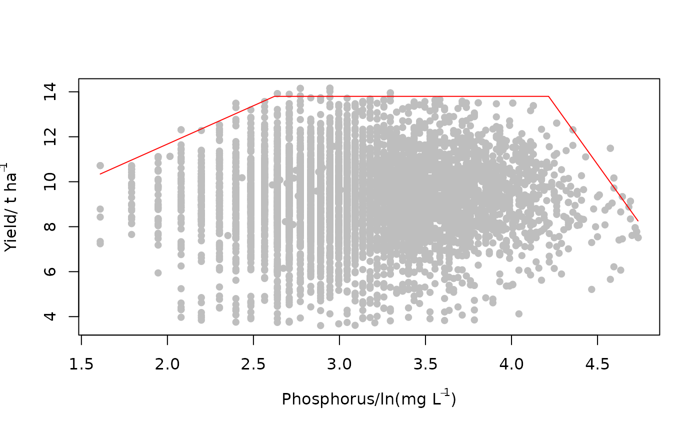
Trapezium model ("trapezium") $$y={\rm min}(\beta_1+\beta_2x, \beta_0, \beta_3 + \beta_4x)$$ where $\beta_1$ is the intercept one, $\beta_2$ is the slope one, $\beta_0$ is the maximum response, $\beta_3$ is the intercept two and $\beta_3$ is the slope two.
Mitscherlich model ("mit") $$y= \beta_0 - \beta_1*\beta_2^x$$ where $\beta_1$ is the intercept, $\beta_2$ is a shape parameter and $\beta_0$ is the maximum response.
Schmidt model ("schmidt") $$y= \beta_0 + \beta_1(x-\beta_2)^2$$ where $\beta_1$ is ascaling parameter, $\beta_2$ is a shape parameter (x-value at maximum response ) and $\beta_0$ is the maximum response .
Custom model ("other") This option allows you to create your own model form using the function function(). The custom model should be assigned to the argument equation. Note that the parameters for the custom model should be a and b for a two parameter model; a, b and c for a three parameter model; a, b, c and d for a four parameter model and so on.

The function bolides() utilities the optimization procedure of the optim() function to determine the model parameters. There is a tendency for optimization algorithms to settle at a local optimum. To remove the risk of settling for local optimum parameters, it is advised that the function is run using several starting values and the results with the smallest error (residue mean square) can be taken as a representation of the global optimum.

The common errors encountered due to poor start values

function cannot be evaluated at initial parameters
initial value in 'vmmin' is not finite

References

Nelder, J.A. 1961. The fitting of a generalization of the logistic curve. Biometrics 17: 89–110.

Phillips, B.F. & Campbell, N.A. 1968. A new method of fitting the von Bertelanffy growth curve using data on the whelk. Dicathais, Growth 32: 317–329.

Schmidt, U., Thöni, H., & Kaupenjohann, M. (2000). Using a boundary line approach to analyze N2O flux data from agricultural soils. Nutrient Cycling in Agroecosystems, 57, 119-129. Schnug, E., Heym, J. M., & Murphy, D. P. L. (1995). Boundary line determination technique (BOLIDES). In P. C. Robert, R. H. Rust, & W. E. Larson (Eds.), site specific management for agricultural systems (p. 899-908). Wiley Online Library.

Author

Chawezi Miti <chawezi.miti@nottingham.ac.uk>

Examples


x<-log(SoilP$P)
y<-SoilP$yield
start<-c(4,3,13.6,35,-5)

bolides(x,y,start=start,model = "trapezium",
        xlab=expression("Phosphorus/ln(mg L"^-1*")"),
        ylab=expression("Yield/ t ha"^-1), pch=16,
        col="grey", bp_col="grey")

#> $Model
#> [1] "trapezium"
#> 
#> $Equation
#> [1] y = min(β₁ + β₂x, β₀, β₃ + β₄x)
#> 
#> $Parameters
#>      Estimate
#> β₁   4.853076
#> β₂   3.410976
#> β₀  13.796772
#> β₃  58.721169
#> β₄ -10.656856
#> 
#> $RMS
#> [1] 0.2334075
#>